Market Data

August 1, 2016
Gross Domestic Product for Q2 2016- First Estimate
Written by Peter Wright
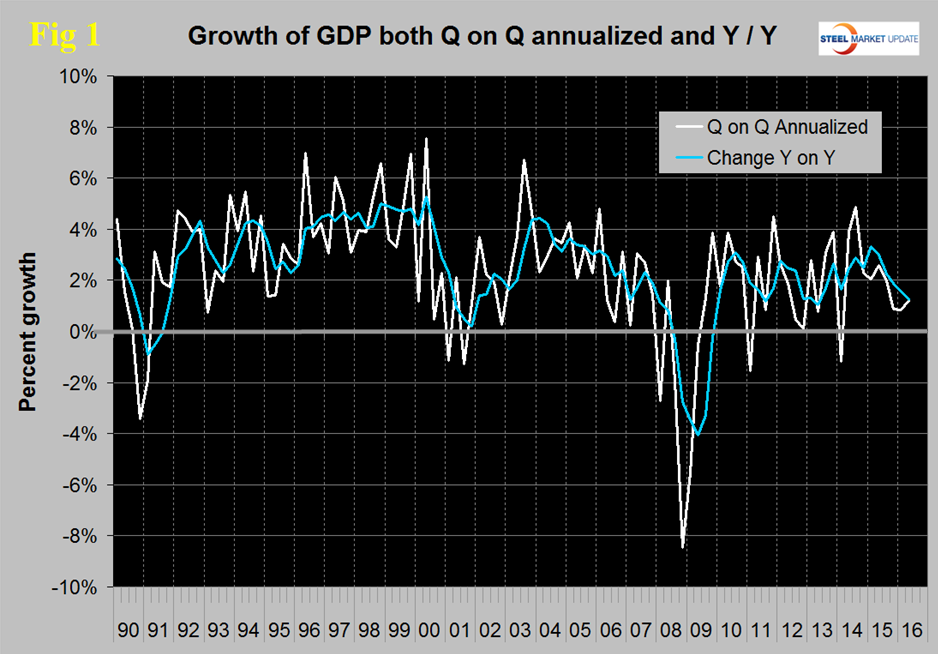
In the Bureau of Economic Analysis report of GDP released on Friday, economic statistics were revised back to Q1 2013. In these revisions, Q2 and Q4 of 2015 were revised down as was Q1 of 2016. Q1 of 2015 was revised up substantially and Q3 of 2015 was unchanged. The annualized GDP growth rate in the first estimate of the 2nd quarter of 2016 was 1.22 percent which was about half of analysts’ expectations. The result for Q1 2016 was revised down from 1.08 percent to 0.84 percent. GDP is measured and reported in chained 2009 dollars and in the second estimate of Q2 was $16.575 trillion. The growth calculation is misleading because it takes the quarter over quarter change and multiplies by 4 to get an annualized rate. This makes the high quarters higher and the low quarters lower. Figure 1 clearly shows this effect.
The blue line is the trailing 12 months growth and the white line is the headline quarterly result. Occasionally these measures coincide which was the case in the latest data. On a trailing 12 month basis, GDP was 1.23 percent higher in the 2nd quarter of 2016 than it was in Q2 2015. In the last six years, since Q1 2011 the trailing 12 month growth of GDP has tracked between a high of 2.88 percent to a low of 1.07 percent therefore the latest result remains within this range at the low side.
Economy.com wrote the following on July 12th: “Why haven’t rock-bottom interest rates led to more growth? Or more precisely, given the strong job market, why haven’t productivity and thus GDP growth been lifted more by the low rates? There are likely many reasons, but a key one may be evident in the pedestrian credit growth since the crisis. Interest rates ultimately impact productivity growth through the credit used to finance investment. Credit also fuels the demand growth necessary to give businesses incentive to invest in expanding their operations. Unlike in past recoveries when credit growth spurted into the double digits, in this recovery it has remained largely fettered in the low to middle single digits. This in turn likely goes to the overarching changes to financial regulation since the crisis, including much higher required levels of capital, greater liquidity, more rigorous risk management via stress-testing and living wills, and substantially greater regulatory oversight. Many of these changes make for a safer financial system, but it has been a tough adjustment for the system, resulting in less credit growth. Interest rates have fallen, but the regulatory burden has increased, resulting in constrained credit growth, investment, and thus productivity and GDP growth. Having said this, it is encouraging that the financial system is well down the regulatory reform path. Regulators have capital and liquidity levels close to where they want them, and financial institutions have largely finished hardening their risk management infrastructures. If so, then the low interest rates should soon translate into a stronger economy—certainly not a weaker one as many observing the currently low rates fear.
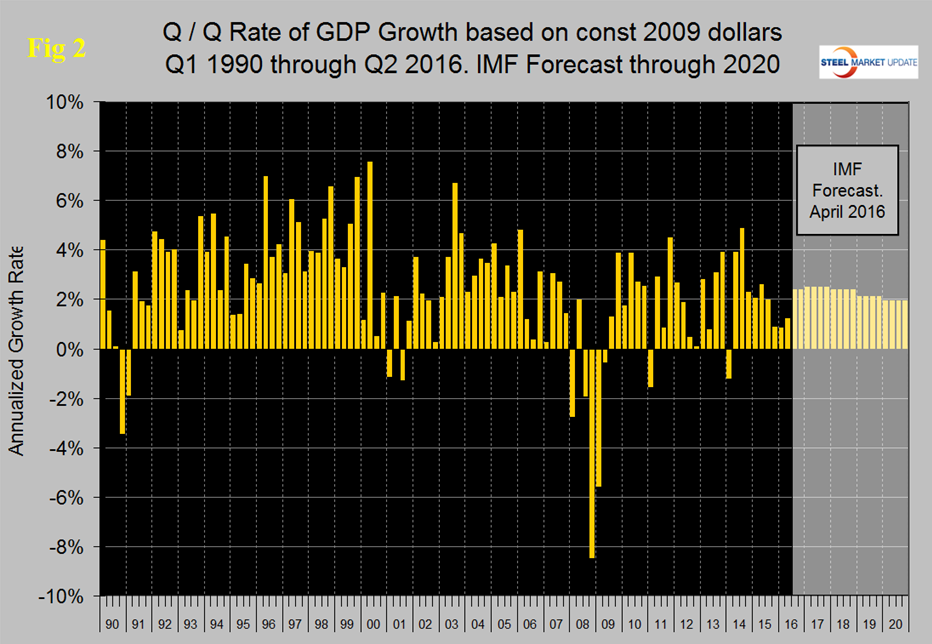
Figure 2 shows the headline quarterly results since 1990 and the latest IMF forecast through 2020. In their April revision, the IMF downgraded their forecast of US growth in 2016 from their October estimate of 2.84 percent to 2.4 percent and downgraded 2017 from 2.80 percent to 2.50 percent. It looks as though the IMF may still be optimistic.
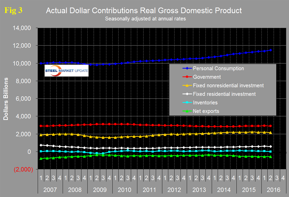
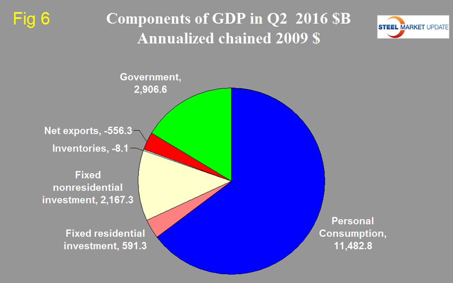
There are six major subcomponents of the GDP calculation and the magnitude of these is shown in Figure 3. Personal consumption accounted for 69.3 percent of the total in the latest data and made the highest contribution to growth since Q4 2014. Retail sales again surprised on the upside in June, suggesting consumer spending growth may be gaining momentum.
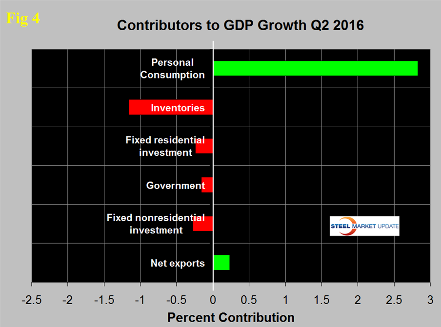
Figure 4 shows the change in the major subcomponents of GDP in Q1 2016 and the dominance of personal consumption as a growth driver.
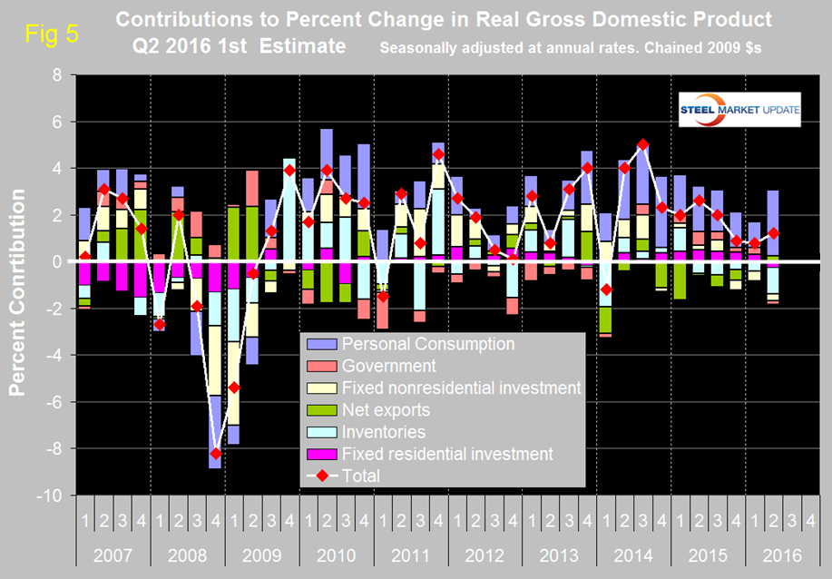
The change in inventories was the greatest detractor with a contribution of negative 1.16 percent. Declining inventories have a negative effect on the overall GDP calculation and this has been the case for the last five quarters. Over the long run inventory changes are a wash and simply move growth from one period to another. Construction, both residential and non-residential which includes infrastructure made negative contributions in Q2 which is at odds with the Commerce Department report of construction expenditures in their CPIP report. The BEA data for GDP is seasonally adjusted and in our CPIP analysis we have a choice to examine either seasonally adjusted or non-adjusted data. We choose to consider only non-seasonally adjusted data therefore we have introduced a discrepancy in government data from different departments. Net exports made a positive contribution in Q2 and added 0.23 percent. Since US trade is net negative we don’t understand this result but we reproduce here what was reported. Figure 5 shows the contributors to GDP extended back through Q1 2007 and describes the quarterly change in the six major subcomponents.
In this latest data the negative contribution of inventories was the greatest since Q1 2014. The contribution of personal consumption at 2.83 percent was up from 1.11 percent in the 1st Q and the highest since Q4 2014. Personal consumption includes goods and services, the goods portion of which includes both durable and non-durables. Government expenditures contributed negative 0.16 percent in Q2 down from positive 0.28 percent in Q1. The contribution of fixed residential investment at negative 0.24 percent was the first time that this component detracted from GDP since Q1 2014. The contribution of fixed nonresidential investment has been negative for three consecutive quarters. Figure 6 shows the breakdown of the $16.6 trillion economy.
SMU Comment: Historically it has been necessary to have about a 2.5 percent growth in GDP to get any growth in steel demand so this latest estimate of GDP doesn’t suggest any improvement in steel demand in the immediate future. This relationship is a long term average and in reality steel is extremely more volatile than GDP. If GDP takes a dive then steel demand craters and if GDP takes a sudden upturn steel soars. Neither of these extremes is evident at present. We have observed frequently in our SMU reports that steel demand has not been where it should be based on several previously indicative benchmark indicators and that a decline in inventories throughout the supply chain was probably a major contributing factor. This GDP data would seem to be supportive of that view as an inventory reduction has detracted from GDP since H1 2015.


